Similar Words ... an Easy Intro to Vector Spaces

In the last post we did some fun stuff, based on the idea of word co-occurrence to indicate some kind of similarity or connectedness in meaning.

What we found was that word co-occurrence worked well for generating sentences - great fun - but was plagued by the boring word (stop word) problem. Lots of words co-occur with the boring word "and" .. but that doesn't mean those words are all somehow related to "and" in meaning.

So let's try another approach that's a teeny weeny bit more sophisticated. And exploring this will lead us to another great tool used by professional text data scientists.

Similar/Related Words

What do we mean when we say two words are similar. We weren't that precise before. Here are some options:

• One word causes another  .. e.g. virus causes disease
• One word is a kind of another .. e.g. a horse is a kind of a mammal
• One word is just another way of saying the other .. e.g. lazy is almost interchangeable with idle

There are other kinds of ways words can be related or similar .. but for now let's focus on the third kind above ... where words have the same, or almost the same, meaning .. and could be swapped out for each other without too much trouble.

Of course real language is subtle and complex .. so the words umpire and referee are almost the same but one is actually used in preference to there other depending on the sport... a football referee and a cricket umpire. This particular complexity is one we'll embrace rather than ignore...

Meaning Comes From Context

How do we know whether a word is similar to another. Well we could look them up in a dictionary and compare definitions. That's not a stupid idea at all! But dictionary definitions are actually not that comparable .. and we'd still have to automatically interpret those definitions ... which takes us back to the original problem of getting computers to understand human language.

Let's try again...

Have a look at the following diagram which shows three words car, van, and banana.

The words are linked to other words that they co-occur with. So the word car co-occurs with the words seats, drive and take. That's what you'd expect .. nothing controversial here.

Now if you look at the word van you can see it shares a lot of the co-occurring words with car .. again, you would entirely expect this. That's because the two things, car and van, and very similar ... they act similarly, they are used similarly, built similarly and can often be used interchangeably.

But there are ways in which a van is different from a car. The above shows that the word height is sometimes used with van but rarely or not at all with car.

Now the word banana .. well, that word doesn't share any co-occurring words with car or van .. except maybe the word take it shares with car.

So this diagram allows us to see which words are similar in meaning or use, without even having to use a dictionary to actually understand what the words really mean! We do it simply by spotting the shared context of the related words.

That's pretty powerful!

There's more! ... 

The words car and van don't co-occur much ... yet the above diagram shows that they are similar through their shared neighbours!

... That's really powerful!

Uses of Finding Similar Words

The uses for finding similar words are huge! Off the top of my head, we could:

• find words that were similar to ones we had
• documents that were related to others (which contained enough similar words)
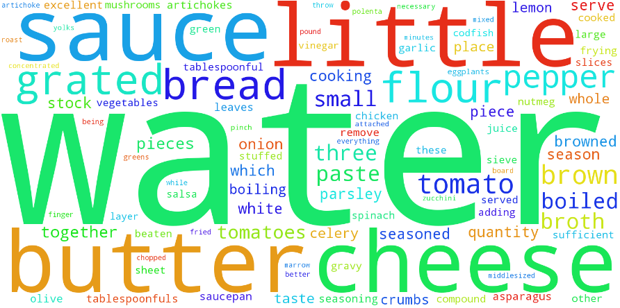
• visually cluster similar words to understand what an unknown text was about quickly without having to read all the text
• find new words, or uses of words, in a corpus .. and understand how they were used
• ...

Exciting!

How Would We Do It (By Hand)?

Let's now think about how we would find similar words, following the above idea of shared co-occuring words.

We should certainly use the matrix of co-occurrences that we built last time. That gives us the co-occurrence of one word following another.

When we talked above about co-occurrence we din't care about word order .. so we'd need to change. that matrix a little bit. We'd have to sum the values for word1 -> word2 and word2 -> word1 because that gives us the co-occurrence irrespective of which word comes first. Easy enough!

Now, imagine we have a word car ...  how do we use that matrix to find similar words? Remember, we mean words that are similar because they share lots of co-occuring words.

Have a look at the following diagram of a co-occurrence matrix:

What's the word that's the most similar to car? Let's take this slowly and step by step.

Let's see if the word fish is the answer. Remember - we're not looking at simple co-occurance of fish and car. We're looking for other shared co-occurent words.

• If you look across from car you can see which it it is most co-occurent with - wheels, paint.
• If you look across from fish, it is most co-occurent with nothing much else.
• So car and fish don't share much co-occurrent words.

Let's see if the word van is the answer.

• If you look across from van, we can see it is mostly co-occurrent with wheels, paint.
• That's the same set of words that are most co-occurrent with car, which we just did above.
• That means car and van share lots of co-occurring words. 

Yay! That means car and van are similar!

Ok - that's great, how do we turn this into some kind of calculation that a computer can do?

How Would We Do It (By Computer)?

Let's look back at what we did above by hand. We looked across from each candidate word, and considered which words were most co-occurrent with that candidate word ...

... And if those co-occurrent words matched ... then the two words were similar. Similar according to our definition above.

How do we calculate such commonality? Well, if you look again at that matrix above, the darker matrix cells have higher values .. and it's those we wanted to match. The following diagram shows this more clearly:

Between car and fish, there aren't dark cells that line up. Between car and van there are, as shown by the green arrows.

Numerically, we could multiply the values. This is simple .. which we like ... and seems to have the right outcomes. If there are low vales in the cells we want to match .. the multiple is low. If both are high the multiple is high .. which is what we want. And, crucially, we try to match a high value with a low value .. we get a lowish value too .. which is what we want.

Let's see this in action, with calculations done in a spreadsheet:

Yup - seems to work as we want. The high valued multiples only happen if both multiplied values are high .. that is a match for co-occurring word.

Then we simply sum up the multiples, representing the matches, ... to get a score for similarity. Here we have a similarity score of 0.01 for car and fish ... makes sense. And we have a score of 1.76 for car and van ... also makes sense!

So we now have a computer method for finding similar words! .. wasn't such hard work!

Getting Fancy - Word Vectors And The Spaces They Live In

You've probably heard loads of people talking about using vector spaces to do fancy stuff with words. They certainly give the impression that this mysterious stuff is kind of magic and powerful!

Let's demystify it a bit!

First of all - there are many different ways vectors and vector calculations are used .. there isn't only a single way. We'll start with just one.

If you look at that calculation we just did .. we multiplied the cells of a sequence of cells. All of the numbers in a row are associated with the word we're interested in.

So you can see that the row of numbers is a vector (of numbers) for the word in question. Here's the vector for the word car:

$$ \mathbf{car} =
\begin{pmatrix}
1.00 \\
0.90 \\
0.00 \\
0.80 \\
0.20 \\
0.00 \\
\end{pmatrix}$$

So similarity score is the dot product of these vectors ... which is a nice coincidence, because the dot product sums the multiplies of the corresponding vector elements - precisely what we've done above to calculate the similarity score!

$$ \mathbf{similarity} = \mathbf{word_1} \cdot \mathbf{word_2}$$

This is also great because many computer programming languages or their supporting libraries make dot products of vectors easy and efficient. That includes Python too!

Let's take a different look at what this dot product does. First let's see what that vector really is, and where it lives:

Each element in those vectors is a magnitude along an axis. An axis that represents the co-occurence word. So the space that these vectors live in is the space of co-occurence words. It's nice to think of this space as a space of themes, or topics, or ideas, or meanings...

Taking the dot product of two vectors in this space is the same as measuring the angle between them (the maths is easy).

$$\mathbf{a \cdot b} = |a| \  |b| \ \mathbf{cos}(\theta)$$

If the vectors are normalised to 1, this super simplifies nicely to

$$\mathbf{a \cdot b} = \mathbf{cos}(\theta)$$

You can think of that dot product as a measure of similarity ... a smaller angle means the vectors are more aligned, and $\mathbf{cos}(\theta) \to 1$ ... a bigger angle means they are point in very different directions and are not similar, and $\mathbf{cos}(\theta) \to 0 \to -1$.

Next Time

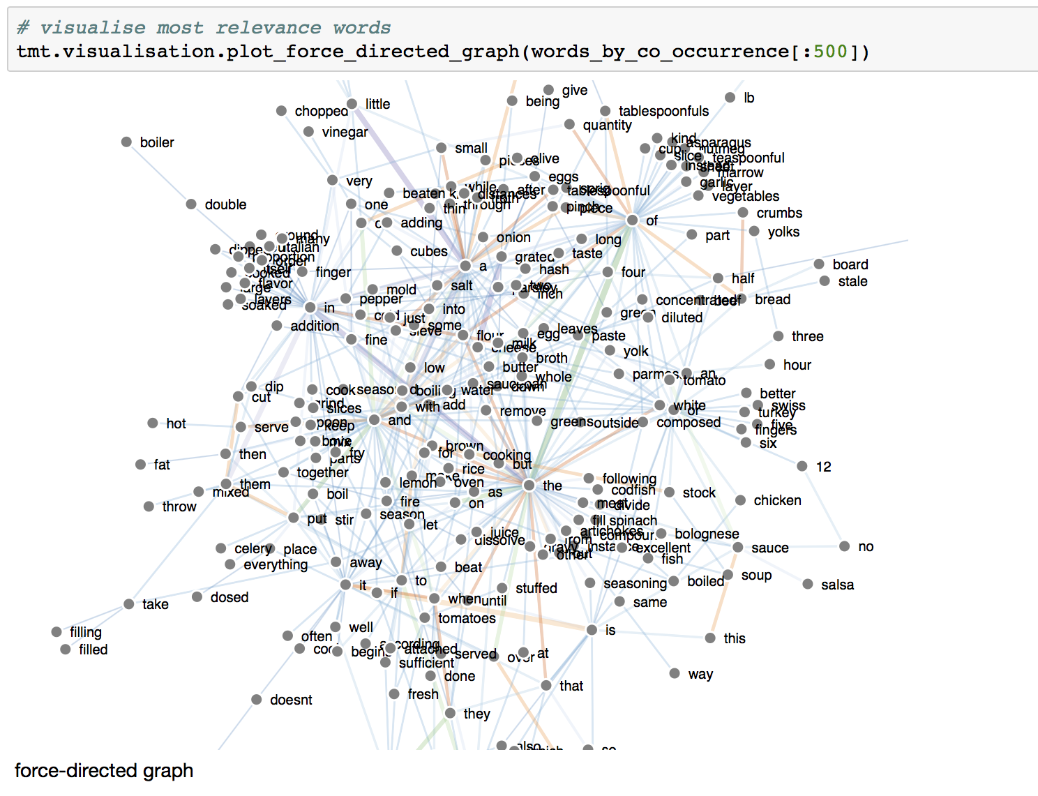
Next time we'll implement these ideas and see how well they work. We can look forward to seeing if we can:

• recreate the force-directed graphs based on this new measure of similarity (based on commonality of co-occurrent words)
• cluster similar words based on this similarity
• cluster similar documents
• search engine based - not on exact matches - but on similar words, where similarity is this new definition

Fancy Terminology

Here's some fancy terminology you might hear others using about some of the stuff we talked about here:

• 2nd order co-occurrence ... that's just the definition we developed above .. where we consider how much of word1's co-occurrent words are the same as those for word2. We saw how van and car are themselves no co-occurring but they are similar because they share many common other co-occurring words. Second order just means "once removed" here .. as shown in the diagram earlier.

• vector space - a space in which vectors exist ... the focus is on how we define the axes. There are all kinds of vector spaces, and above we made one which had axes of co-occurrent words. 

Co-Occurrence .. and Generating Sentences

Most of our work has looked at words on their own. We know that meaning is often in the context of a word, so we must look around any single word to try to capture this contextual meaning.

There are several ways of doing that - some of them fairy sophisticated. But for now, we'll start super simple, as usual, and grow from there, ready for the more complex stuff later.

Co-Occurrence: Words That Occur After A Word

Let's start by considering which words occur after a given word. So for example, if I thought about the word "apple", maybe the word "pie" is most likely to occur after this. If I think about the word "Iraq" maybe the word "war" is most likely to appear next.

We kinda looked at this when we broke a corpus into 2-grams and counted how often they occurred. We're going to do the same sort of counting again but a bit differently because we want to later build on the approach we develop here. It will become clear why we're doing it differently, I promise!

Let's jump into the (not very deep) deep end! Have a look at the following table.

Let's decode what this is. You can see down the left words like "apple", "pie" and "fish". These have been labelled word1. That was easy enough.

You can also see across the top a similar thing, words labelled word2. What the numbers in the table are showing is how likely the second word2 is right after word1 in a given corpus. Fair enough.

What are the numbers inside the table? Those are the likelihoods that word1 is followed by word2. The illustrated example is "apple" followed by "pie" ... as in "apple pie" ... which has a likelihood of 0.99 out of a maximum of 1.0. That's very high - which means that apple is very likely to be followed by pie. Makes sense again ...

Often such matrices are symmetric - but that's not the case here. The word "pie" is not likely to be followed by the word "apple", and it shows in the table as a low likelihood of 0.05. It's not zero because our text cleaning might strip punctuation and so the word apple might actually be the beginning of a new sentence of sub-phrase.  Again this all makes sense .. apple pie .. not pie apple.

The actual numbers used here are probabilities between 0 and 1. We could have chosen another kind of measure, like word count, which is simpler. Remember from earlier though, word count is easily biased by bigger documents, so maybe a more normalised measure like word frequency is better.

We could even use the measures of interesting-ness (TF-IDF) we developed earlier to moderate these probabilities ... that way we de-emphasise words like "the" and "a" which will dominate co-occurrence. But for now let's keep it simple.

So what can we do with such tables of co-occurrence values?

1. Identify Insightful 2-Word Phrases

We could take the word pairs with the highest co-occurrence value and see if they give us any insight into the corpus. Here's the top 20 for the mini Italian recipes corpus we use for experimenting with:

	word1	word2	co-occurrence
0	of	the	19.0
1	with	a	17.0
2	in	the	16.0
3	a	little	16.0
4	grated	cheese	16.0
5	salt	and	15.0
6	it	is	14.0
7	in	a	13.0
8	them	in	13.0
9	the	fire	12.0
10	and	pepper	10.0
11	and	put	10.0
12	on	the	10.0
13	they	are	10.0
14	oil	and	9.0
15	to	be	9.0
16	over	the	9.0
17	tomato	sauce	8.0
18	with	the	8.0
19	butter	and	8.0

This is just like taking the top 20 n-grams by word count that we did before. That's ok - remember we're doing it this way because this way can be extended to new ideas .. hang in there!

We can see that only a few of the top 20 word pairs are actually that insightful ... most of the words are what we previously called stop word - boring and not unique. We'll try applying the uniqueness factor later.

If we didn't know what a corpus was about, bringing out the top 20 2-grams like this helps us understand that it might be about food or recipes.

2. Generate sentences!

This is going to be fun.

Imagine we pick a word at random .. we can use that table to look up the most likely next word. We're going from word1 to word2. Fine, nothing special here.

But if we then take that second word, and use it as the first word, we can find the most likely next word .. a third word. If we repeat this, we ca get a whole sequence of words.

Maybe we'll get meaningful sentences? Let's try a few ... the following shows sequences of 7 words (we could do more, or less) with deliberately chosen first words.


      the fire with a little more and pepper
      once into the fire with a little more
      then cut them in the fire with a
      olive oil and pepper and pepper and pepper
      tomato sauce salsa bianca this sauce salsa bianca
      cut them in the fire with a little
      cook in the fire with a little more
      little more and pepper and pepper and pepper

So for a first go ... that's kinda spookily good! Some of the sentence seem to be fairly well formed, and actually very much on topic!

Because we're not doing anything more sophisticated (we could) we do fall into traps like word sequences that keep repeating like "olive oil and pepper and pepper and pepper".

Phrases like "cook in the fire with a little more" are pretty impressively natural!

We should be really pleased with this - a super simple technique - and we get spookily good results!

3. Graphs of Word Nodes Linked by Co-occurence

This is also kinda cool .. and open up lots of possibilities that we'll explore later.

If we take the word pairs with the highest co-occurrence values, and plot them as connected nodes, the resulting graphs can be interesting, beautiful, and hopefully insightful too ... because we can see which words are connected which other words, and whether some words are the nexus of many others .. and in some way central to the meaning of the corpus.

Let's try it with the small Italian Recipes corpus. We developed force directed graphs in the last post and they've been improved to have word labels, colours, and also wider links for larger co-occurrence values ... click on the following to enlarge it.

Well .. it's busy! It's the top 500 word pairs by co-occurrence value. You can also see that there is some structure .. with some words clustered around what must be important words. Either drag a node, or hover over it, to see what the word is.

As we half-expected, many of the central words are actually those stop-words .. those boring words that aren't that insightful. The words "in", "of", "the" are at the centre of quite a few clusters. That's ok - we're just starting to explore using graphs .. we can find ways of removing or reducing them, be using stop-word exclusion lists or using the TF-IDF measure of interesting-ness we developed earlier.

Before we do that - have a look at just the following graph which only shows those pairs which have a co-occurrence above 3 .. in an attempt to remove noise and concentrate on those pairs for which there is lots of evidence for that pairing.

That's much clearer if we're busy and don't have time to explore a graph of loads of nodes.

Code

As usual the code for both the data processing pipeline is in a notebook on github:

• https://github.com/makeyourowntextminingtoolkit/makeyourowntextminingtoolkit/blob/master/04_co-occurrence_graph.ipynb

And the code for the visualisation is also on github, the following sows the library function and the d3 javascript:

• https://github.com/makeyourowntextminingtoolkit/makeyourowntextminingtoolkit/blob/master/text_mining_toolkit/visualisation.py
• https://github.com/makeyourowntextminingtoolkit/makeyourowntextminingtoolkit/blob/master/text_mining_toolkit/html_templates/d3_force_directed_graph.js

Next Ideas

This is a great start ... and we've developed a powerful (and pretty) visualisation too! Here are some of the ideas we can try next:

• Use stop-word removal or TF-IDF measures to reduce importance of boring words. 
• Extend co-occurence beyond just two words .. maybe 3, 4 or even much longer sequences ... suitably adjusted so that closer words are still given a higher score. This will deal with language which often places important words around a boring word like "apple and pear" ... "fish in the oven" ... 

Interactive D3.v4.js in a Jupyter Notebook

One of things we want to develop is a visualisation for word co-occurance .. that is, a measure of how often words appear one after another.

A good way of doing this is with a graph of nodes, kinda like the following:

You can see how each node can represent a word, and the links between nodes (words) can be coloured or widened to indicate how often one word is followed by the next.

It would also be great to be able to play with the elements, to shift them around or zoom into a big graph.

D3.js

There is a really popular javascript library for creating rich and interactive visualisations called d3. Check out their gallery to get a feel for the really cool, and interactive, visualisations it can make. There's even more here ... I can't get enough of them!

Here's an example of an live interactive graph at bl.ocks.org .. have a go at dragging the nodes around.

You can see it constantly reshapes to maximise the visibility of each node, whilst trying to maintain the links between them.

Problem: D3.v4.js in a NoteBook (from a Library)

Plotting images and charts in a notebook is easy and has been done for a long time. You may already know about matplotlib, the de-facto library for plotting in a notebook.

Working with d3.js is slightly different because it is a javascript library - that means it needs to work in the browser. Normally tools would work behind the scenes in the engine (notebook kernel) and once the results were created, they would be pushed to the browser to be displayed. Javascript libraries don't do that - the do the work in the browser.

So d3.js plots are created in the browser. How do we do that with a jupyter notebook?

Luckily, there is a fairly mature method for executing HTML and Javascript in a notebook cell. Here's a super simple example:

You can see how an object is created from the raw HTML, and then this object is "displayed" .. or rather executed. That's cool!

You can find more examples of executing rich media in a notebook cell here ... including examples showing how javascript can be executed in a browser notebook.

If we're developing a toolkit visualisation library, we don't want the user to type all that stuff into a cell and then execute it. That would defeat the point of a library that takes all the details away.

Can we run the above python in a library function, for the results to be displayed in a notebook? Yes, we can!

Here's a basic library function which does the HTML mangling so the notebook user never sees it:

import IPython.display

def test_html(s):
# create html object
h = IPython.display.HTML(s)
IPython.display.display_html(h)
pass

And here is what it looks like ... nice and simple!

That's how we want to use d3 ... by getting a library to do all the HTML and Jascripty stuff. Let's try it:

import IPython.display

def test_html(s):
# create html object
h = IPython.display.HTML(s)
IPython.display.display_html(h)
pass


def test_d3():
html_string = """
<svg width="400" height="200"></svg>

<script src="https://d3js.org/d3.v3.min.js"></script>
"""

js_string="""
console.log(d3);

var svg = d3.select("svg");

var circle = svg.append("circle")
   .attr("cx", 100)
   .attr("cy", 100)
   .attr("r", 40)
   .attr("fill", "blue")
    .attr("stroke", "black");

"""

h = IPython.display.HTML(html_string)
IPython.display.display_html(h)

j = IPython.display.Javascript(js_string)
IPython.display.display_javascript(j)
pass

You can see how we use d3 to select the SVG HTML element and then create a circle inside it.

Here's what happens:

Ok .. that didn't work! Seems like d3 isn't visible from the python library when used in a notebook. hmmm... even more weird is if you just hit it again, it works:

That's not inspiring confidence .. and anyway we want to work with d3.v4 not d3.v3 ... let's see what happens if we change the source URL to point to https://d3js.org/d3.v4.min.js:

A similar error, and this one doesn't go away like the other one did by repeatedly calling the function.

So we have a problem to fix. It might be tempting to work with the d3v3 weird behaviour - but we won't, we'll press ahead and look to the future with the new d3v4 ... we don't want to be locked into an ancient version of a library. And anyway, we want to fix the problem properly if we can, not reply on some wobbly workaround.

Diagnosis

I'm not an expert but after a week of wrestling with this ... and terrible documentation ....

The problems seem to be due to a different way that the d3.v4.js library presents itself to whatever it is loaded into.

The v3 version seemed to create a global reference, so anyone could see and call it. That doesn't appear to be the case for v4 .. Again, I'm no expert, but I think it is trying to be clever and present itself based on what it thinks the host environment is ... and it gets it wrong when the host is a Jupyter notebook.

The various tickets on this seem unanswered - e.g. http://stackoverflow.com/questions/39335992/d3-4-0-does-not-create-a-global-d3-variable-when-imported-into-jupyter-notebook

To make things worse, browsers and/or the notebook seem to cache previous javascript libraries .. making you think things are working when they're not .. or are broken when they're not! To properly test this I needed to close down a browser properly and kill all history/cookies/cache.

My Solution

Here's how I finally got it to work.

The key is to use the require.js method to load the d3 library and remove the <script> method of loading the library. The Jupiter notebook already makes use of require.js so we don't need to load that. Note the lack of a ".js" at the end of the URL.

require.config({
    paths: {
        d3: "https://d3js.org/d3.v4.min"
    }
});

require(["d3"], function(d3) {
    // do stuff here
}

So let's try it ...

That works! .. and with version 4 of the D3 library too!

Here's a preview of work in progress developing an interactive force-directed graph for word co-occurance .. you can see the node "pear" highlighted. You can't see here, but we can drag the nodes about and let the graph rebalance.

Reference Code

Here's sample reference code for getting d3v4.js working from a Python library invoked by a Jupiter notebook:

import IPython.display

def test_html(s):
# create html object
h = IPython.display.HTML(s)
IPython.display.display_html(h)
pass


def test_d3():
html_string = """
<svg width="400" height="200"></svg>
"""

js_string="""
require.config({
    paths: {
        d3: "https://d3js.org/d3.v4.min"
    }
});

require(["d3"], function(d3) {

console.log(d3);

var svg = d3.select("svg");

var circle = svg.append("circle")
   .attr("cx", 100)
   .attr("cy", 100)
   .attr("r", 40)
   .attr("fill", "green")
   .attr("stroke", "black");

});
"""

h = IPython.display.HTML(html_string)
IPython.display.display_html(h)

j = IPython.display.Javascript(js_string)
IPython.display.display_javascript(j)
pass

Multi Word Search Queries

We've already developed a simple way of searching an index to see which documents contain a word.

We even refined the way we want the search results, first prioritising the documents which the highest word count, and then by using our more sophisticated relevance measure.

The challenge now is .. how do we handle queries with more than one word?

More Than One Query Word

Let's have a think about this. Imagine we have 3 documents and an small index of only 3 words, shown here:

You can see, for example, that the word rice doesn't appear in doc1. You can see that it appears in doc2 with a high relevance score. Doc1 seems to feature cake a lot!

What do we want to happen when we give our computer a search query with more than one word - say "rice cake"? That's not a simple question. So let's take it slow.

We don't want our toolkit to ignore one word or the other. That's why we provided both. Good - that's a start, at least.

Do we want our toolkit to consider each word on its own, and return the two sets of results? So we could see the scores for the word rice, and note that doc2 came top, and similarly see that that doc1 came top for the word cake. We could then .. maybe order doc1 above doc2 because the score for cake was 0.5, higher than the 0.4 for rice.

Well ..  that could work, and it's not a terrible start ... but why did we provide two words in the first place? Because we wanted to find results which were related to both words together.

That's our first clue as to how to handle the query. We want to prioritise documents which are related to both search query words - both "rice" and "cake" in our example.

How do we do this? Well. we could look at an index based on 2-grams and try to find "rice cake" in there. That's actually a very good answer - but fails if the two words are not always right next to each other. And anyway, we often find ourselves having to work with an index of 1-grams not 2-grams, or 3-grams, etc ...

Let's have another go using the 1-gram index above. Could we combine these scores in some way that reflects our intention when we issues the search?

Combining Scores

As always, let's start with the simplest thing we can do, and only make things more complex if we really really need to.

A very simple thing we can do is simply add the scores that each query word has for a document.

Have a look again at the index:

Using the words rice and cake:

• doc1 has a combined score of 0.0 + 0.5 = 0.5
• doc2 has a combined score of 0.4 + 0.1 = 0.5
• doc3 has a combined score of 0.3 + 0.3 = 0.6

So this means doc3 wins! ... not doc2 which had the highest score for rice alone, and not doc1 with had the highest score for cake.

You can see how, doc1 might have been abut cakes, but maybe not rice cakes. And doc2 might have been a rice dish but not rice cakes.

So let's try this idea of adding relevance scores for each search word in a query ... often called search terms.

Code

The code to implement this is really simple .. which shows you the power and ease of Python and pandas.

# query string to list of search terms
search_query_list = search_query.split()

# do query
documents = relevance_index.loc[search_query_list]

# sum the scores
results = documents.sum()

# filter out those with score of zero
results = results[results > 0]
return results.sort_values(ascending=False)

The query is still a simple lookup of the index data frame. The sum is also really simple. The results can contain zeros (word not present) so we get rid of those, again very simple. We finally sort the results in descending order, so the highest scores are first.

Results

Let's try it and see what happens:

• A search for "saffron rice" places 05.txt top for both indices. That's good because it is in fact the recipe for "rice with saffron".
• A search for "bread soaked in milk" results in both indices returning 17.txt and 03.txt which both contain bread (crumbs) soaked in milk. But the relevance index returns 00.txt as the top result. This is not ideal, especially as the document doesn't contain the word milk but is boosted because the document contains a high concentration of the word bread. 

That second observation suggests we need to refine the combination of scores. We'll come back to this later, as we've made a good start for now.

Results from Improved Word Relevance Measure

In the last post we looked at improving the early measure of relevance which was based on word count.

Word count works well, but suffers from bias due to long documents (more words), and also from rewarding lots of boring words (the, it, a, is, to ...).

Let's see how well it all worked.

Finding Interesting / Boring Words Automatically

If we apply the measure to the recipes data set, we should be able to identify the boring (stop) words automatically. These will be the ones with the lowest relevance scores.

Previously, the most frequent words for a recipes corpus was full of boring words. The first interesting word "oil" appeared at position 13, after 12 boring words ranked higher! Here they are again for easy reference:

   the        273   

   and        203   

   a           133  

   with        79   

   for         77   

   in          72   

   1           58   

   to          56   

   of          49   

   2           44   

   then        43   

   until       41   

   oil         41   

Relevance scores for a word are per-document. But we can sum them up across all documents. Here's what the words with the top 10 look like (shown with their relevance scores)

[('sauce', 0.072479554515290895),

 ('them', 0.070833510080924769),

 ('little', 0.062832341904529035),

 ('rice', 0.058276255134080412),

 ('butter', 0.057278834991103734),

 ('bread', 0.055933326383546908),

 ('they', 0.054793552703163897),

 ('quantity', 0.051914014707442335),

 ('together', 0.050062707525060902),

 ('grated', 0.048860949578921925),

 ('broth', 0.048693197257887351),

 ('tomato', 0.048444379129175236),

 ('boiled', 0.047588072543957513),

 ('flour', 0.047404394383271695),

 ('water', 0.046392876975336547),

 ('then', 0.046343005577901039),

 ('pepper', 0.044368328433798621),

 ('some', 0.044303584017951085),

 ('very', 0.043970962688707774),

 ('that', 0.043831469829911401)]

Much much better! That top 20 contains lots of interesting words with only a few we would consider not so interesting. There are no short boring stop-words like "a", "in", "to" .. so our measure which penalises shorter words works well!

Let's see what the bottom 20 look like ... these should be the boring words:

[('and', 0.0),

 ('in', 0.0),

 ('the', 0.0),

 ('up', 0.0012725563329122366),

 ('i', 0.0012816579235383377),

 ('bit', 0.0017987306071704534),

 ('had', 0.0017987306071704534),

 ('now', 0.0017987306071704534),

 ('1', 0.0020042948378737836),

 ('3', 0.0020042948378737836),

 ('4', 0.0020042948378737836),

 ('2', 0.0020042948378737836),

 ('32', 0.0020148808604443747),

 ('leaf', 0.0022240465989832267),

 ('your', 0.0022240465989832267),

 ('wet', 0.0022988261123030452),

 ('top', 0.0022988261123030452),

 ('pie', 0.0022988261123030452),

 ('than', 0.0024192873309550364),

 ('line', 0.0024192873309550364)]

Yup - these are all boring .. except maybe leaf.

For a method that didn't rely on manually providing a list of stop words, this approach works really well. And it'll adapt to different corpuses, as each will have different word usage.

Here's a word cloud based on these relevance scores.

Compare that with our previous best word cloud:

What we're seeing is two different pictures - the first tries to show words that are interesting per-document, the second shows words that are prominent across the corpus. Both of these approaches are useful when exploring text.

Notebook on Github

All the code is on github. The notebook for this pipeline is at:

• https://github.com/makeyourowntextminingtoolkit/makeyourowntextminingtoolkit/blob/master/03_index_and_search.ipynb

Challenging Texts

Some text corpora are more challenging than others. The word clouds for the Iraq War Chilcot Report and the Clinton Emails data sets have not been that illuminating ... because they'e filled up with words that appear often but aren't that interesting. Here's a reminder of what they looked like before:

Let's see how our attempt at reducing the impact of boring words works. Remember, this means reducing the impact of words that appear often but in all documents, making them less "unique".

You can see that the Iraq Report word cloud has new and interesting insights - multinational, resolution, basra, baghdad, de-ba'athification, map, inspectors, intelligence, did  witness, weapons, ... much more insightful than the more expected words we had before. Interestingly, the words iraq, report and inquiry are in the bottom 20 for relevance (interestingness).

Let's try the Clinton emails which were really very challenging because the emails are fairly informal, lack continuity or strucure, and full of un-polished prose.

Well, we can see that we no longer have boring words like state and department, unclassified and date, subject and sent. You'll recognise these as words you find in the raw text of all emails - they're not that illuminating .. so our relevance measure really works to penalise them. Great!

What else does that word cloud show - well it brings forward key dates, 2009, 08-31-2015 and 06-30-2015. If you were investigating the emails, these would be worth looking into. As it happens, these are the dates the emails were released, so not that interesting for us .. but they could have been.

Identities pop out too. Abedin is a close advisor and aide to Clinton - you can read about here: http://www.vanityfair.com/news/2016/01/huma-abedin-hillary-clinton-adviser. Cheryl and Mills are the same person, Cheryl Mills, another aide: http://www.politico.com/story/2015/09/cheryl-mills-hillary-clinton-aide-213242. The same for Jacob Sullivan https://en.wikipedia.org/wiki/Jake_Sullivan

A few key email addresses also pop out .. including hrod17@clintonemail.com and hdr22@clintonemail.com ... apparently secret email accounts she is alleged to have used inappropriately for official business: http://www.factcheck.org/2015/05/clintons-secret-email-accounts/

Search Relevance

Let's see how search result ranking changes with this relevance measure. The following shows the results of searching for the word "king" in Shakespeare's Macbeth.

Searching the basic word count index gives:

macbeth_act_01_scene_02.txt    14.0
macbeth_act_01_scene_04.txt     7.0
macbeth_act_01_scene_03.txt     6.0
macbeth_act_01_scene_06.txt     5.0
macbeth_act_04_scene_03.txt     4.0
macbeth_act_05_scene_08.txt     3.0
macbeth_act_03_scene_01.txt     3.0
macbeth_act_01_scene_05.txt     3.0
macbeth_act_04_scene_01.txt     2.0
macbeth_act_03_scene_06.txt     2.0
macbeth_act_02_scene_03.txt     2.0
macbeth_act_03_scene_02.txt     1.0

Searching the relevance index gives:

macbeth_act_01_scene_02.txt    0.010196
macbeth_act_01_scene_06.txt    0.006776
macbeth_act_01_scene_04.txt    0.005312
macbeth_act_01_scene_03.txt    0.001888
macbeth_act_01_scene_05.txt    0.001810
macbeth_act_03_scene_06.txt    0.001803
macbeth_act_05_scene_08.txt    0.001636
macbeth_act_03_scene_01.txt    0.000935
macbeth_act_03_scene_02.txt    0.000807
macbeth_act_04_scene_03.txt    0.000759
macbeth_act_04_scene_01.txt    0.000627
macbeth_act_02_scene_03.txt    0.000605

Both ways of sorting the search results give is Act 1 Scene 2 as the first result. If we have a look at the actual text, we can see why .. it is a key scene with King Duncan.

But the second place result is different. The relevance index places Act 1 Scene 6 second, whereas the basic word count give sis Act 1 Scene 4. Both involve the king, but scene 6 is shorter and is mostly about the king's arrival speech, so is less "diluted".

The fact that very similar documents appear in the top, albeit in a different, order suggests we're not wilding off with the new relevance measure.

Summary

Basic word count is a good way of working out what a text is about. Given it's extreme simplicity, it's power is pretty amazing.

But where it falls down, we can use a refined measure - we call it relevance - which counters the bias of longer documents, penalises short words, and promotes the uniqueness of a word too.

We should use both measures as part of our toolkit, as this relevance measure can diminish words which really are relevant but happen to be prevalent in the text corpus.